Learn the basics about R² and RMSE in the article here
R² and RMSE are two common statistics you’ll need to use to understand your devices’ performance, but on their own, both of these metrics have important shortcomings. In this article you’ll learn how to put them together, along with knowledge about the pollutant you are measuring to draw useful conclusions about your sensor performance.
While R² is the most commonly used accuracy metric and is often found in “rankings” that evaluate air quality sensors, it should not be used in isolation as it does not take into account the range of pollutant concentrations that the devices are exposed to during the test: Since R² expresses how well the device under analysis measures changes in pollutant concentration compared to the reference instrument, this metric doesn’t work well when there is no significant change to evaluate on.
To demonstrate the sensitivity of R² on the range of pollutant concentrations, please refer to actual field data from a Clarity Node and a collocated reference monitor (image below). The R² is 0.86 for the full dataset. However, when a filter is applied and only the concentrations below 20 𝞵g/m3 are analyzed, the R² drops to 0.65 (see the figure below). Note that we are evaluating the same sensor, so ideally it should not receive different accuracy scores depending on the range of pollutant concentrations used to test it.
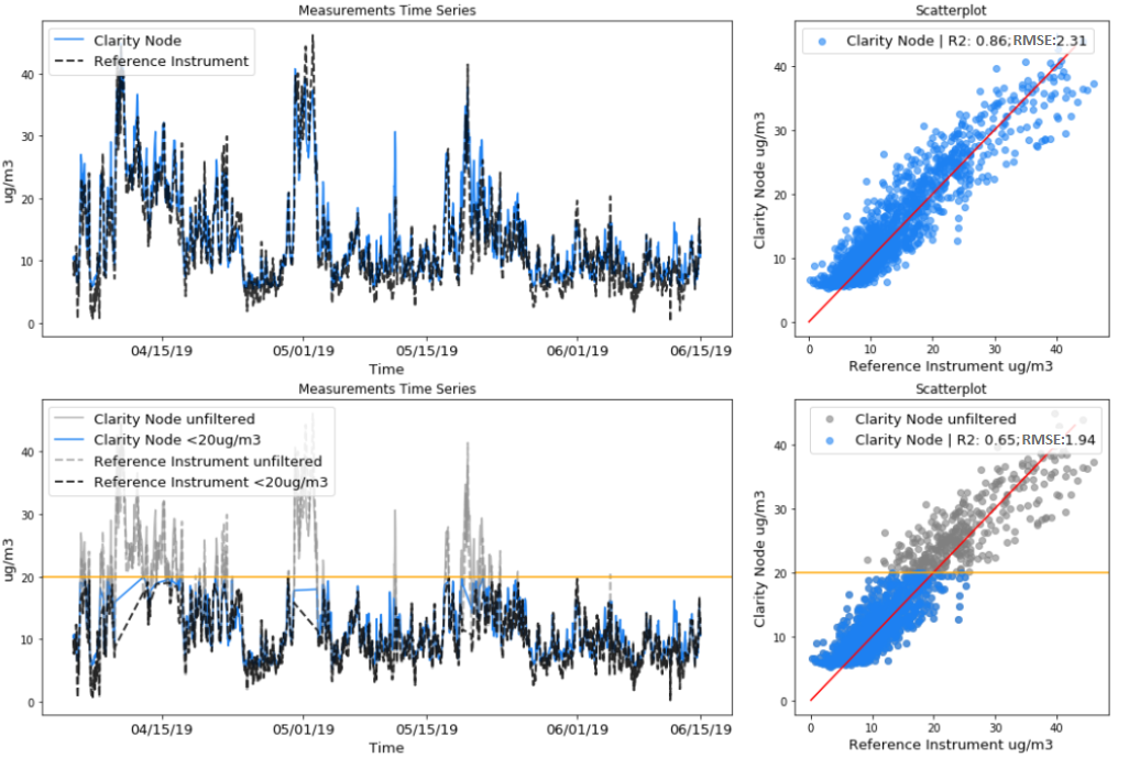
Top: Measurements time series and scatterplot for a Clarity Node and a reference station that are measuring PM2.5 over time. Bottom: same plots but whenever the Clarity Node reads above 20 𝞵g/m3 the data is filtered out.
A second limit of the R² metric is that it only evaluates the ability of the device under analysis to detect relative changes in pollutant concentrations. The ability of the device under analysis to output the same value as the reference instrument is not taken into account. If you rely on the R² in isolation, you might assume that a sensor is performing well while missing the fact that the sensor is overestimating pollutant concentrations, like in the example shown in the image below.
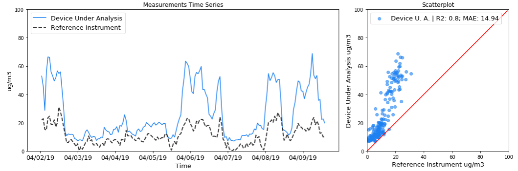
Measurement time series and scatterplot for an imaginary device under analysis and reference instrument that are measuring PM2.5 over time. Example of good R² score and pollutant concentration overestimation.
Similarly to R², also RMSE has limitations and should not be used in isolation: the RMSE metric does not tell us whether deviations can be corrected through calibration, or are caused by random errors and sensor limitations which cannot be corrected. All kinds of deviations increase RMSE equally. A sensor with a high R² that perfectly tracks changes in pollutant concentration, but is off by a factor potentially due to a poor calibration, might have a similar RMSE to a broken device that always outputs the same number. Luckily, a high R² can point to the possibility of calibrating the device under analysis.
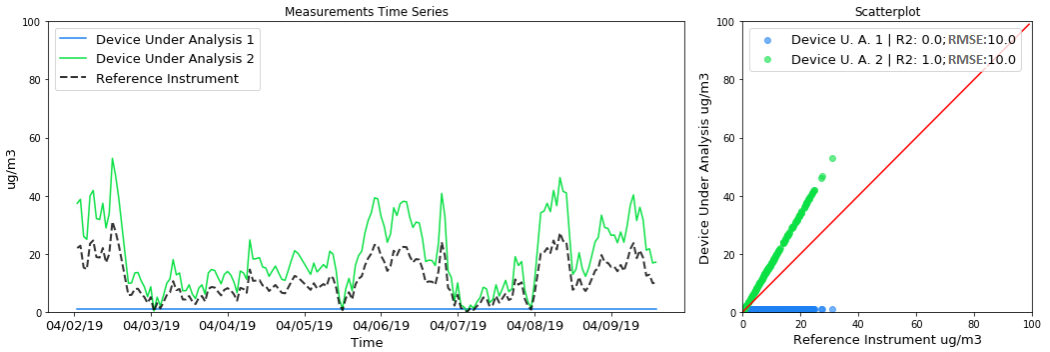
Measurements time series and scatterplot for two imaginary devices under analysis and reference instruments that are measuring PM2.5 over time. One device is uncalibrated, the other is broken. Both devices have the same RMSE.
Furthermore, similarly to R², also RMSE is affected not only by sensor performance, but also by the range of pollutant concentrations over which the sensor is evaluated: Evaluating a sensor over a high pollutant concentration range may result in a high RMSE, but low relative error.
To avoid the pitfalls of R² and RMSE, Clarity recommends using them in tandem and not in isolation. To learn how to do that, let’s imagine we are evaluating two sensors as shown in the two figures below:
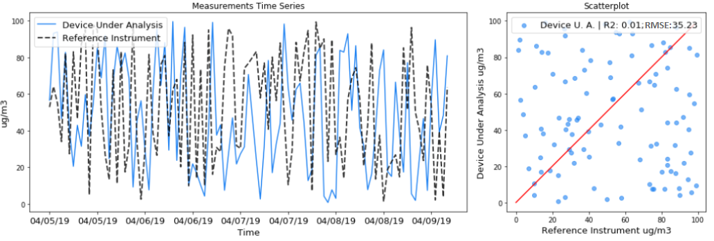
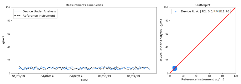
Both graphs report low R² close to 0. On the top graph, RMSE is equal to 35.23 𝞵g/m3, in the bottom one RMSE is equal to 1.76 𝞵g/m3. Note that the y-axis range purposefully kept from 0 to 100 in both graphs to show the difference in the two datasets.
Once we calculate R² and RMSE for each sensor, we can add our knowledge of pollution phenomena to the analysis. For the imaginary sensor that generated the top graph, no correlation with the reference instrument is observed (R² = 0.0). Furthermore, the average deviation between its measurements and the reference measurements (RMSE) is 35.23 𝞵g/m3. We know that such deviation could lead to severe misclassification of air quality. This means that the device should be regarded as inaccurate for the purpose of monitoring ambient air quality.
For the imaginary device that generated the bottom graph, no correlation with the reference instrument is observed (R²= 0.0). However, the average deviation between its measurements and the reference measurements (RMSE) is less than 2 𝞵g/m3. We know that a deviation of 2 𝞵g/m3 is not significant compared to the bigger changes in pollutant concentration we are trying to observe. This means that, in principle, the device might be able to correctly classify air quality, and the low R² could be the result of a low range of pollutant concentrations during the test. This is substantiated also by the time series chart, which looks like a flat line with concentrations never exceeding 10 𝞵g/m3). In this case, it is recommended to repeat the test with a wider pollutant concentration.
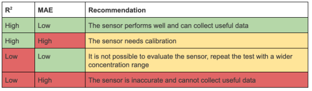
In this section, we have learned about the limitations of R² and RMSE, and each tells us something about our sensor's ability to accurately measure air pollution. To summarize how to use R² and RMSE in tandem to evaluate sensor performance, refer to the image below: